High-Tech Software House
(5.0)
This is a real-life case study from our project related to image processing and computer vision - in fact, we will show in this post how we managed to achieve its performance acceleration.
The image processing project and the challenge
Autonomous driving is a hot topic in today's industry, representing the technological revolution we are witnessing. However, the autonomy of vehicles is a complex problem with many ambiguities, including control theory, simultaneous localization and mapping (check out our previous post) and a high-level understanding of the environment, which will be our main concern in the following post.
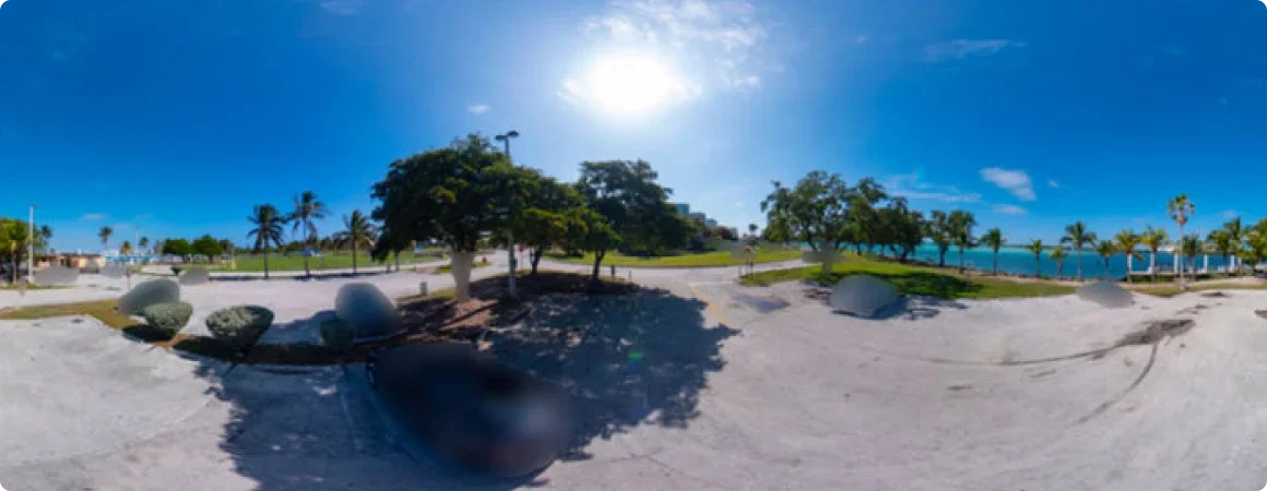
Nowadays, one of the most popular applications of computer vision in autonomous driving is to blur people's faces and vehicle registration plates in the camera image of road-mapping cars. All this ensures that the General Data Protection Regulation (GDPR) provisions are not violated. However, panoramic photos are large, and processing might take a while before we obtain a result, so the main challenge to overcome is to reduce that time. Our case study begins with a system in which processing a single image took about ~3 minutes, which did not meet real-world deployment requirements. The images (360° photos) were 20,000 x 10,000 pixels, and 70% of the processing time was occupied by convolutional neural networks for object detection and segmentation. Initially, the Mask R-CNN model inference was run solely on the CPU using OpenCV with OpenCL backend.
Proposed approach
Our goal was to speed up the application and, more specifically, the Mask R-CNN's inference so that the processing of photos would be faster and more efficient. In addition, speeding up could not mean a deterioration in the application's capabilities. We split our work into three components.
One of the most popular ways to decrease the memory consumption of a graphics card is a technique called quantization. That is a process of taking all parameters in the neural network model, i.e., weights, biases and activations, and converting them to some more miniature numerical representation, e.g., from float32 to int8. Reducing the number of bits in the memory taken by all parameters might affect the scale of an entire model, which might contain millions of parameters. To allow for full FP16 throughput, remember to set the DNN_TARGET_CUDA_FP16 next to the DNN_TARGET_CUDA as preferable target and preferable backend in code. We are aware that the internet is full of tutorials on OpenCV installation, so make a long story short about installing OpenCV with CUDA support follows these bullet points:
Cmake output of the OpenCV project should look similar to the picture below. When the project is generated, just build it and install.
It’s worth mentioning that DNN_TARGET_CUDA_FP16 can decrease GPU memory consumption and increase processing speed. However, the latest is tricky because there are some GPUs where FP16 is slower, and be sure to check it out here. In the following post, we focus primarily on the inference of the existing model. Still, the numerical precision of the model’s parameters is a broad topic that also affects the training procedure, its speed and achieved performance. More on improving training using different precision settings can be found here.

The following section presents two C++ programming tricks that speed up the implementation of so-called image mixing. But what is that? Image mixing in our application is a situation in which we have a binary mask of detected objects in the original image. We want to apply a blur operation only to these regions. To sum up, we have two images: the original one and the blurred one, with binary masks in which blurring pixels must reside in the resulting image.
Originally, the solution involved iterating over the entire (a very large and panoramic) image over rows and columns using two for loops, and deciding which pixel has to be “blurred, and which has to stay original. That solution was correct, however far from optimal, and resulted in very poor performance. The following psued-code represents the original solution for the image-mixing problem.
In contrast with the original implementation, our approach focuses on only one loop over raw pixels’ pointers, i.e. rows, columns and channels. In such an approach, we use OpenCV only to get the starting pointer, and the rest of the processing is written in pure C++. First, direct access to the memory together with no nested loops improves the speed of image mixing. Moreover, the operation itself does not require any floating-point arithmetic. Instead of blurring regions, we use only uint8 multiplication and uint16 division, which yields an additional factor that speeds up the application. The algorithm could be implemented using the following pseudo-code.
The fast implementation of image mixing has some drawbacks significant to software developers:
The fast implementation works out of the box when we work on full panoramic images. However, when we apply it only to some Regions of Interest (ROI), clone that ROI first, as in the code snippet below.
The clone operation creates a new image from ROI and stores it in a different memory location. Without that, there is no copying, and the pixel’s pointer stays in the original image. Due to that, iteration over the memory differs from iterating over the pixels of the ROI.
The Gaussian Filter and the Box Filter are well-known and widespread filters extensively used in various vision-based applications. They are both low-pass filters, which reduces the amount of high-frequency noise in the input signal (images are also signals). Visually in the image, their application gives the blurring effect. Both filters include kernels with specific weights that are applied to the image using convolution (see the great visual explanation of different types of that operation). See the picture below to compare the Gaussian kernel, in which weights follow the Gaussian distribution, and Box Filter’s kernel, where weights follow a uniform distribution.


But how do the filter’s weights correspond to the image processing? The 2D convolution operation is generally an element-wise multiplication followed by summation. In the case of the Box Filter, each weight is 1, so the filtering reduces only to averaging pixels covered by a kernel. In the case of Gaussian filtering, we need to apply each weight to the corresponding pixel, an operation that does not exist in the Box Filter. Additionally, the box filter achieved a similar anonymizing effect as the Gaussian filter with 2x smaller kernel size. Therefore not only do we get rid of multiplication, we also have a lower number of additions. Migrating the blurring process to GPU and Box filtering additionally boosted the processing speed.
In the following post, we presented a three-stage approach that allowed us to speed up our vision-based application. We focused on the practical side of the solution, pointing out algorithms that cannot be considered low-hanging fruits.
Before changes, the application needed ~3 minutes to process one image, and the inference of a neural network occupied 70% of this time. After changes made by Flyps experts, the time it took for neural networks decreased to 9 seconds. Thanks to the applied changes, the application has been accelerated by 20 times.
If you have any questions about this blog post that you would like to ask our experts or would like to talk about what we can do for you, don't hesitate to get in touch with us via the form or via e-mail: [email protected].
See our tech insights
Like our satisfied customers from many industries